The code base for this project can be found here and here

For the final project of my Bayesian Robotics class, the only requirement was to come up with a practical implementation of some of the concepts that were taught in the class. As such, my partner and I had an idea to implement real-time risk mapping and tracking for autonomous robots using only a depth sensor similar to the one found on the Microsoft Kinect. Both static and moving objects would be detected, with the static objects having a fixed region of high risk surrounding the object that the robot will want to avoid. For moving objects, the movement of the object itself is tracked and predicted. Once the velocity and direction of the object is found, we can predict where the moving object is likely to be in the near future. This likelihood region maps directly to the areas where we would like the robot to avoid. To achieve this, we used the Asus Xtion Pro sensor along with OpenNI and OpenCV for data acquisition and processing. Qt was chosen as the cross-platform framework for the front-end GUI.

Background

Copied from our report:

As the trend moves towards replacing humans with robots in dangerous environments, many of the behavioral decisions that are instinctively made by humans are often overlooked when implementing robotic AI. Examples of these behavioral decisions include risk analysis, object recognition, and pathing optimization. While these decisions are often made by the pilot in manually controlled robots, autonomous robots often lack these details in their decision making logic. Risk analysis in particular stands out as one of the more complex behavior to model due to its non-deterministic nature. Many factors must be taken into account when creating such complex models. These factors include the merging of data from various sensors of different complexity and dimensions, deriving the current operating state while taking its past history into account, and creating a complex map of possible options where the surroundings are changing.

Here we present a basic implementation of risk analysis where areas of high risk are mapped out through the use of IR and distance sensors. The risk regions for moving objects vary in shape and size depending on the object’s motion, and is derived using a motion model associated with the moving object. Our implementation uses the data from a cheap sensor that is widely available to draw a risk map of a room given the objects in its field-of-view. In addition, the motion path of moving objects are predicted using the same data set.

In an ideal scenario, the robot will have the capabilities to do both room and risk mapping as well as object tracking and motion prediction. In our scenario however, due to limited time, we only implement object tracking and motion prediction. While we are using only one sensor, data from multiple sensors of various types can be easily combined to create a full layout of a robot’s surrounding area. We assume that this capability to create a map of the surrounding area is preimplemented on all autonomous robots.

The Hardware

Originally we had planned on using the ubiquitous Microsoft Kinect for our project, but we ended up finding a few small issues with the device that made it significantly harder to use. The first major issue with the Kinect was its requirement for a 12V power source. As we wanted to power everything off of either the robotic platform or a laptop placed on the platform, the Kinect would have required more time that we didn’t have to add a step-up regulator and other circuitry. The second issue was the size and weight of the device; the first-generation Kinect is actually quite large at 12″ x 3″ x 3″ and heavier at almost 3lb. To get around these issues, we decided to instead go with the Asus Xtion Pro. Both the Xtion Pro and Kinect are comparable in terms of sensor specifications as they both use the same underlying sensor developed by PrimeSense. The Xtion Pro however, is much smaller at 7″ x 2″ x 2″ and only weighs 0.5lb. In addition to the smaller size and weight, the Xtion Pro is powered solely off a USB port, making integration into an existing system a trivial task.

The Kinect and Xtion Pro have nearly identical sensor specifications. The official specifications for the depth sensor are as follows:

• Distance of use: 0.8m to 3.5m
• Field of view: 58° H, 45° V, 70° D (Horizontal, Vertical, Diagonal)
• Depth image size: VGA (640×480) : 30fps, QVGA (320×240): 60fps

In our testing, we found that the actual usable distance ranged from 1.0m to 6.7m. The error however, increases exponentially with increased distance. Shown in the images on the right, we can see that the returned depth values from the sensor correspond linearly to the actual distance of the object. The measurement error however, increases significantly for points that are further away. This is shown to have an impact later on when motion detection is executed on the depth data.

One thing to note is that the sensor does also include a regular RGB camera in addition to the IR depth sensor. Since our aim is to do motion detection and tracking, we only used the depth sensor for our project as it is easier to track individual objects given depth data than with an RGB image. Tracking objects using only a RGB camera is much harder as objects with the same color will be recognized as a single entity. The data from the RGB camera could certainly be used to augment the data from the depth sensor, but we leave that as an exercise for anyone who wants to use our project as the basis for their own work.

Motion Tracking with Depth Data

Depth data is first acquired from the sensor using the APIs from OpenNI. The depth data is returned as a 16-bit single channel value for each pixel. Only ~13 bits of the depth data is actually useful due to the distance limitation from the sensor. These raw values are then converted to the native image format used by OpenCV (cv::Mat) and then passed to another thread for the actual processing. The application utilizes multiple threads for improved performance, with a thread being dedicated to the GUI, data acquisition, and data processing. An excerpt of the data acquisition code is shown below.

In the depth processing thread, we run OpenCV’s background subtraction, morphological operations, and blob detection to track moving objects. For each new frame of data, we execute the following:

1. Update the frame with the latest valid data (not all pixels are valid due to distance/IR shadow/etc).
2. Execute background subtraction using OpenCV’s BackgroundSubtractor algorithm.
3. Run morphological operations (opening following by closing) to remove noise and fill holes in the mask.
4. Average the movement mask’s values over a few frames and erode the results by a bit to ignore object edges.
5. Compress the resulting data into a horizontal plane and draw resulting image.
6. Draw movement points and run OpenCV’s SimpleBlobDetector algorithm to find center of object.
7. Filter object’s center through a Kalman Filter and calculate object’s velocity and direction from past values.
8. Drawing resulting velocity and direction vector onto the image.

An image is generated at each step detailed above and is made available for display on the GUI. An excerpt of the data processing code is shown below.

The results of this implementation is shown in the video at the end this post. Moving points are marked with a large red circle, and blob detection is executed on the red areas to detect individual moving objects. The center of the blob is shown in yellow, while the green dot shows the average over the last ten frames. The blue dot shows the predicted position of the object from the Kalman Filter along with a vector showing the estimated velocity and direction of the object. Furthermore, I wrote some code to assign a unique persistent ID to each moving objects which is displayed alongside of each object.

Object Position and Movement Prediction

My partner worked on this particular area, so I won’t delve too much into the details here. As we now have the capability to track and predict an object’s movement, we can use this information to calculate the forward reachable set (FRS) of the object, or in layman terms, the probability of where the object will be in the near future.

The FRS for any moving object is going to look something like the above due to Newton’s first law of motion (the concept of momentum). If an object is moving in a given direction at a decent velocity, the likelihood of it suddenly stopping or changing directions prior is very low. This likelihood decreases the faster the object is moving, and increases with longer periods in between measurement updates. The image above shows the likelihood of where an object is predicted to be at a given velocity and an increasing period of time in between updates. Areas where there is a high probability for the object (and thus higher risk) are shown in red, while blue areas indicate low positional likelihood for the object. The blue areas should actually extend quite a bit more, but we have it cropped a bit for easier visualization. The chart shows the different between fast sampling rates on the left and slow rates on the right. A fast sampling rate results in a much smaller likelihood region for the object as the predicted region is corrected more much frequently. As the sampling rate decreases, the object’s positional uncertainty increases.

This prediction has a number of possible uses. As mentioned earlier on, this generated likelihood region directly corresponds to the risk region of a moving object. By calculating the risk region for the robot itself along with moving objects in its field of view, we can combine the risk regions and update the robot’s pathing if any intersections are detected. As shown in the above image, fast moving objects will cause regions that the robot will want to path around to avoid collisions. For our project, we didn’t get around to generating an actual movement path for the robot but pathing can easily be implemented using the A* search algorithm and recalculated with each updated frame.

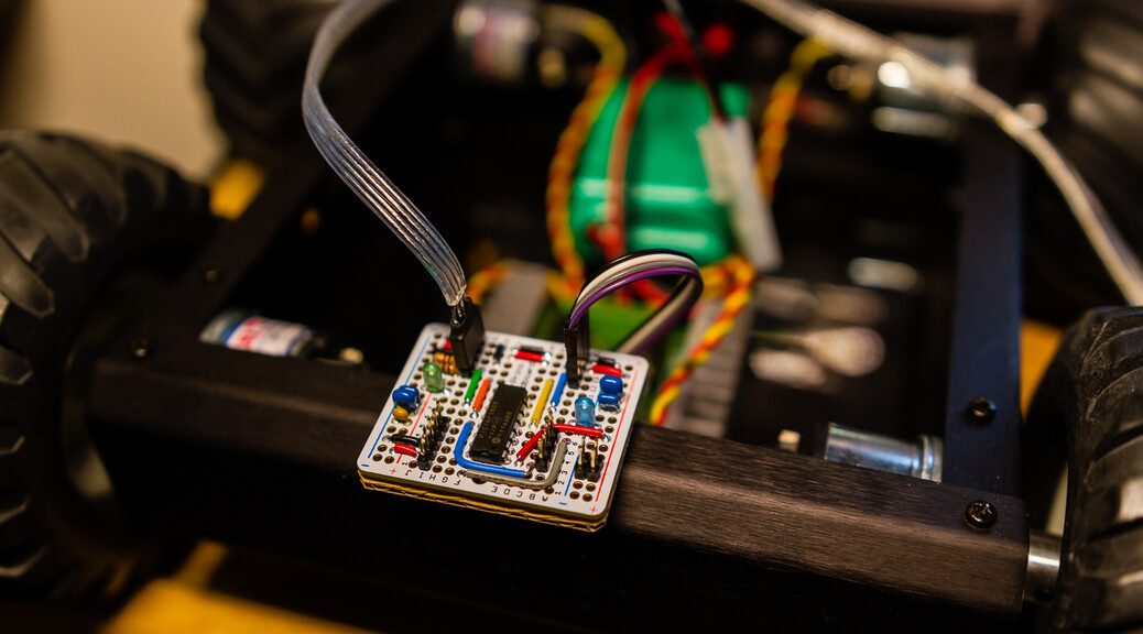
Robotic Platform

While we didn’t get around to implementing autonomous controls, I did put together a basic platform with remote control capabilities. The platform itself was comprised of a A4WD1 base from Lynxmotion along with a Sabertooth 2×12 regenerative motor controller. The controller board for the platform was prototyped using a PIC16F1825 and the optional handheld controller uses a PIC16F1829 along with two analog thumb joysticks from Adafruit. The robot controller board polls the handheld controller through I2C and receives commands from a computer using a RN-42 Bluetooth module. The protocols for controlling the robot has been implemented, but the actual autonomous control code was left unfinished due to a lack of time and looming deadlines from other obligations.

Conclusion

As seen from the video below, this implementation works pretty well for tracking moving objects using only the depth sensor data. If I had more time to work on this project, I would’ve liked to add the following features:

• Plotting the predicted object’s position onto the generated map
• Implement SLAM using OpenCV’s SURF implementation
• Increase object detection accuracy using the RGB video feed alongside of the depth data
• Incorporate real-time path generation between two points with risk area avoidance
• Use a lightweight computer (Raspberry Pi) to wirelessly transfer sensor data to a remote computer
• Optimize code to process data at the full 640×480 resolution